This book begins with a simple claim: machine learning is not a separate species of mathematics. It is a way of building mathematical models when the world is messy, the data are partial, and the rules are only partly known.
That matters because many introductions to AI hide the modelling step. They show the learner a dataset, a library call, and a score, as if the central act were pressing “fit”. But before any fitting can happen, someone has to decide what is being modelled, what counts as an input, what counts as an output, what kind of error matters, and what evidence is available. Those choices are mathematics before they are software.
This chapter sets up the modelling grammar for the whole book:
variables and states
inputs and outputs
parameters and predictions
objectives and losses
constraints and assumptions
evaluation and revision
The chapter also points backward into the earlier Wayward House Mathematics path. If any part of the discussion feels slippery, the right response is not to memorise the new vocabulary but to revisit the underlying ideas of functions, sequences, rates of change, and data description.
NoteIn this chapter
Translate a messy situation into a mathematical object (function, distribution, system, decision rule).
Name the pieces: features, targets, parameters, states, and hidden variables.
Choose what “good” means by making loss and evaluation explicit.
Treat constraints (compute, legality, ethics, safety) as part of the model, not an afterthought.
4.1 Guiding examples
Forecasting next-day demand (regression with consequences)
Classifying cases for action (classification as decision support)
Modelling a system with memory (latent state over time)
TipRunning example: Alberta wildfire smoke and station PM2.5
This chapter’s job in the smoke story is to make the modelling object explicit. If you are building a station-based Alberta-first project, write the first draft of a modelling brief now:
Target: next-day (or next-6-hours) PM2.5 at a chosen station.
Features: lagged PM2.5, weather variables, seasonality, and a simple fire-activity proxy.
Hidden variables: mixing height, plume injection, upwind sources, and station representativeness.
Loss story: are smoke peaks worse than ordinary error (asymmetry)?
Evaluation story: what split is honest for events and seasons?
You will reuse this brief in every later chapter, refining rather than replacing it.
4.2 Prerequisite anchors
The most important places to point backward are:
vol-03/04-functions-relations.qmd for functions, inputs, outputs, and composition
vol-04/04-sequences-series.qmd for accumulation, iteration, and changing systems
vol-05/02-differential-calculus.qmd for sensitivity and rates of change
vol-06/04-data-analysis.qmd for summary, variation, and honest description
4.3 From situation to model
A model starts with a situation in the world, not with a formula.
Suppose a town wants to predict next-day water demand. Suppose a hospital wants to estimate the risk that a patient returns within thirty days. Suppose a farm wants to relate weather, soil, and irrigation choices to crop yield. These are different domains, but they share the same structural question:
What mathematical object shall stand in for the part of the world we care about?
That object might be a function, a probability distribution, a dynamical system, or a collection of decision rules. The point is not to mirror reality in full. The point is to keep the aspects of reality that matter for the task and discard the rest.
This is why modelling is an act of selection. We choose:
which quantities deserve names
which quantities are observable
which quantities are hidden
which relationships are treated as stable enough to use
which errors are acceptable and which are costly
A weak model is often not wrong because its algebra is incorrect. It is wrong because it answers a different question from the one the world asked.
4.4 Variables, features, targets, and parameters
The basic language of data science is easier to understand if we place it next to older mathematical language.
In elementary algebra, we write variables such as x and y. In modelling, we still do that, but the variables take on roles.
A feature is an input variable used to make a prediction or decision. If we are predicting electricity use, then outdoor temperature, hour of day, and day of week may all be features.
A target is the quantity we want to predict, estimate, or classify. In the same example, total electricity demand tomorrow might be the target.
A parameter is different. A parameter is not supplied by the world for each new case. It is part of the model itself. In a linear model
\hat{y} = \beta_0 + \beta_1 x_1 + \beta_2 x_2,
the inputs x_1 and x_2 vary from case to case, while the parameters \beta_0, \beta_1, and \beta_2 are chosen during fitting.
This distinction matters all the way through machine learning:
features describe the case
targets describe the task
parameters describe the model
If those roles are mixed up, later ideas such as training, generalisation, and regularisation become much harder to read clearly.
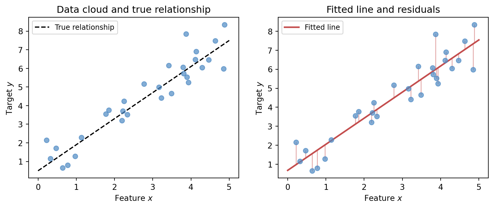
The figure below makes the fitting act geometric. The left panel shows a cloud of observed data and the true relationship (dotted). The right panel adds the fitted line and makes residuals — the gaps between model and data — visible as vertical red segments. Fitting is the act of choosing parameters so that those red segments are collectively small.
Figure 4.1: Left: a data cloud with the true underlying relationship (dotted). Right: the fitted line and residuals (red segments) showing what minimising squared error means geometrically.
4.5 Supervised and unsupervised tasks
One helpful first classification is by the kind of mathematical problem being posed.
In supervised learning, examples come with target values. We are given pairs (x, y) and asked to learn a rule that connects inputs to outputs. Regression and classification live here.
In unsupervised learning, the target is not supplied in the same direct way. We may instead want structure:
clusters in a population
a low-dimensional representation
an anomaly score
a compressed summary of variation
The difference is not merely terminological. In supervised learning the central object is often an approximation to an unknown input-output relationship. In unsupervised learning the central object may instead be a geometry, a density, a partition, or a latent representation.
This means that “learning” is not one operation. It is a family of modelling problems with related habits of thought.
4.6 Models are approximations, not mirrors
The healthiest sentence in this subject is: every model leaves something out.
That is not a weakness unique to machine learning. A line leaves out curvature. A differential equation leaves out microscopic detail. A probability model leaves out the exact future path of a single case. Mathematics becomes useful because it simplifies.
In data science and AI, the danger is forgetting that simplification is a choice. If a model predicts house prices from area, age, and location, then it has already omitted renovation quality, family circumstance, financing conditions, negotiation behaviour, and many other facts. That omission may be reasonable. It may also be the source of systematic error.
So we should ask two questions of any model:
What structure has been retained?
What structure has been discarded?
These questions are more revealing than asking whether the model is “smart”.
4.7 The modelling pipeline as mathematics
It is common to describe the data workflow as a pipeline:
define the task
gather and clean data
choose a model family
fit parameters
evaluate performance
revise
This is often presented as engineering process, but each stage has mathematical content.
Defining the task means specifying the input and output spaces. Cleaning data means deciding what counts as missing, noisy, duplicated, impossible, or incompatible. Choosing a model family means selecting an allowable class of functions or distributions. Fitting means solving an optimisation or inference problem. Evaluation means comparing predictions with reality according to a metric that reflects the purpose of the work.
Even the phrase “model family” is important. We do not usually search over all possible functions. We restrict ourselves to a structured set:
linear functions
trees
kernel methods
state-space models
neural networks
The restriction is not a failure. It is the source of discipline.
4.8 Loss functions make values visible
Once a model produces predictions, we need a way to judge errors. This is the role of a loss function.
If the target is numerical, we might measure squared error:
L(y, \hat{y}) = (y - \hat{y})^2.
If the target is categorical, we may instead use a loss built from predicted probabilities. Later chapters will study these in detail. For now, the key idea is that a loss function is not only a calculation. It is a statement about what kind of mistake matters.
Two forecasting systems can make the same predictions look good or bad depending on the chosen loss. Missing a rare but dangerous event may deserve a heavier penalty than being slightly wrong on many ordinary cases. Overestimating energy demand may be less costly than underestimating it. In medicine, false negatives and false positives often have different consequences.
The loss function therefore sits at the meeting point of mathematics and judgment. It translates purpose into calculation.
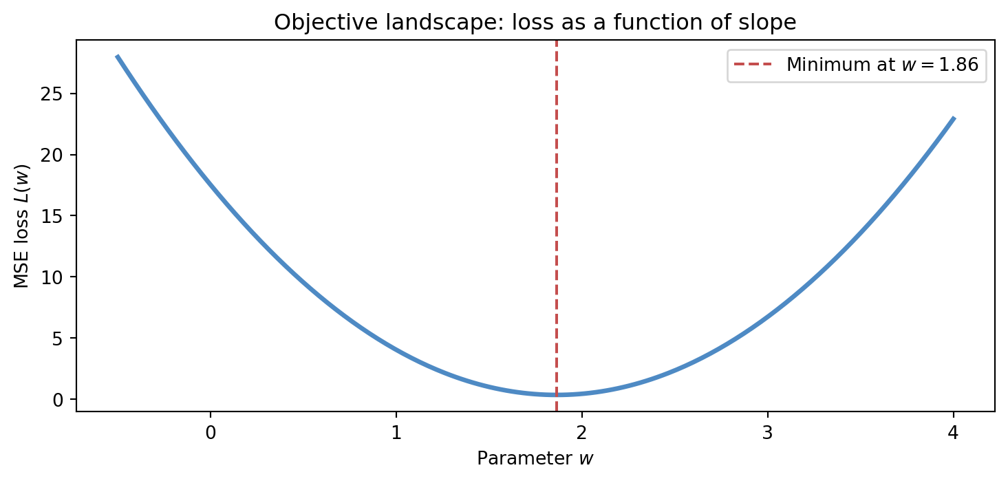
The figure below shows what the loss function looks like as a landscape over the parameter space of a one-parameter model. We hold all data fixed, vary the slope w, and plot the mean squared error L(w) = \frac{1}{n}\sum_i (y_i - w x_i)^2 as a smooth curve. The minimum — the parameter value that best fits the data — is marked by a dashed vertical line. This is the objective landscape, and it will reappear throughout the book whenever we discuss optimisation.
Code
import numpy as npimport matplotlib.pyplot as pltrng = np.random.default_rng(7)n =40x = rng.uniform(0, 4, n)true_w =1.8y = true_w * x + rng.normal(0, 0.7, n)w_vals = np.linspace(-0.5, 4.0, 300)loss = np.array([np.mean((y - w * x) **2) for w in w_vals])w_opt = np.dot(x, y) / np.dot(x, x)fig, ax = plt.subplots(figsize=(8, 4))ax.plot(w_vals, loss, color='#4e8ac4', linewidth=2.5)ax.axvline(w_opt, color='#c44e4e', linestyle='--', linewidth=1.5, label=f'Minimum at $w = {w_opt:.2f}$')ax.set_xlabel('Parameter $w$')ax.set_ylabel('MSE loss $L(w)$')ax.set_title('Objective landscape: loss as a function of slope')ax.legend(fontsize=10)fig.tight_layout(pad=2.0)plt.show()
Figure 4.2: The MSE loss as a function of a single slope parameter w. The curve is smooth and convex; gradient descent follows its slope toward the minimum.
4.9 Training, validation, and test
A model that explains the past perfectly may still fail on new cases. This is one of the deepest practical lessons in modern modelling.
For that reason, we usually separate data into at least three roles:
a training set, used to fit parameters
a validation set, used to compare modelling choices
a test set, held back for final evaluation
This split is not bureaucracy. It is an attempt to protect us from fooling ourselves.
When the same data are used both to build and to judge a model, the assessment is too optimistic. The model has already had the chance to adapt, directly or indirectly, to those examples. A held-out set is a reminder that prediction is a claim about cases not yet seen.
In the earlier series, this resembles the difference between checking an answer against the worked steps you already know and checking whether the method still works on a fresh problem. The second test is harder, but it is the honest one.
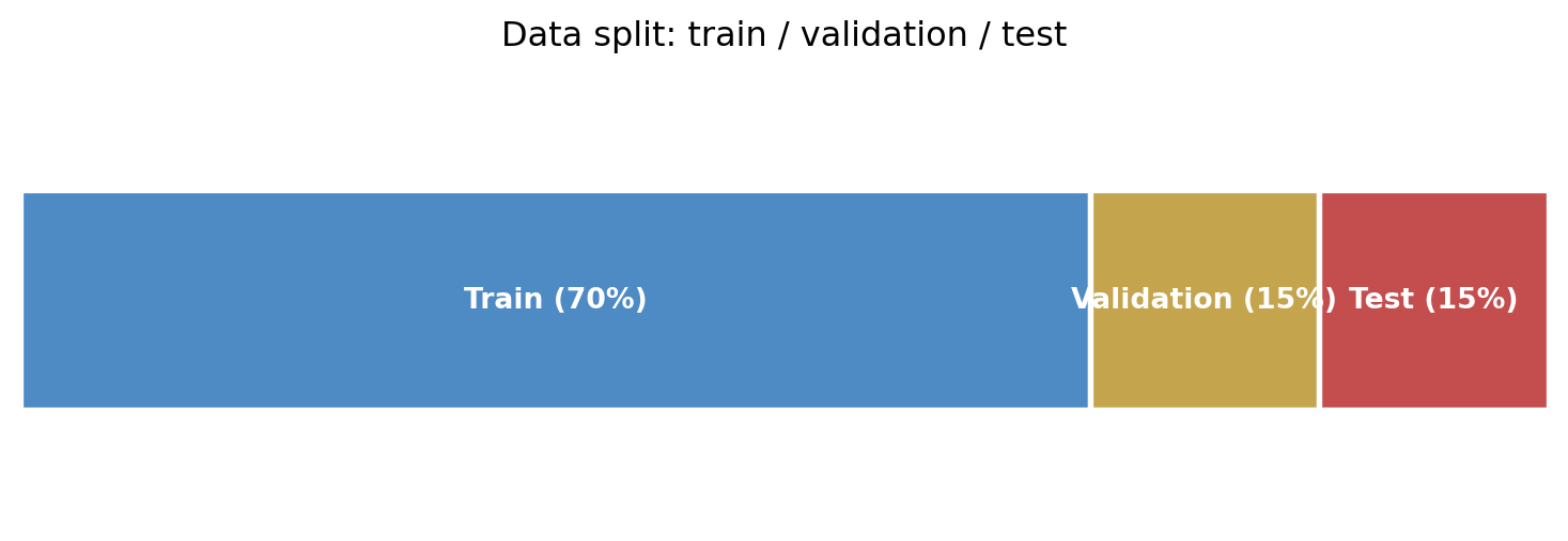
The figure below shows a typical data split as proportional bands. The exact percentages vary by problem size and task, but the structure — a large training region, a smaller validation region, and a held-back test region — is standard.
Figure 4.3: A typical 70/15/15 train-validation-test split shown as proportional bands. The test set is held back until all modelling decisions are finalised.
4.10 A first worked example: predicting demand
Let us sketch a simple modelling problem.
A water utility wants to predict daily demand y for the next day. It records:
average temperature x_1
day-of-week indicator x_2
recent rainfall x_3
yesterday’s demand x_4
One possible model is
\hat{y} = f(x_1, x_2, x_3, x_4; \theta),
where \theta denotes the model parameters.
Even before choosing a specific formula, we can ask good mathematical questions:
Is the target a single number, an interval, or a distribution?
Should day-of-week be treated numerically or categorically?
Is yesterday’s demand enough memory, or is a longer history needed?
Is the error cost symmetric?
Does extreme weather change the relationship?
The purpose of the example is not to solve the whole problem. It is to show that modelling starts with structure. The model is already taking shape before any algorithm is named.
4.11 A second example: classification as decision support
Now suppose the task is to decide whether an email is spam. The target is no longer a continuous number but a label, perhaps y \in \{0,1\}.
The features may include message length, suspicious phrases, sender patterns, and link structure. The model now produces either a class label or a probability that the message belongs to the spam class.
The mathematical shift matters:
the output space has changed
the loss function has changed
the interpretation of error has changed
Misclassifying an ordinary message as spam may be annoying. Misclassifying a malicious message as safe may be dangerous. Again the model is tied to purpose.
4.12 Constraints, assumptions, and hidden structure
Real models live under constraints.
Sometimes the constraint is computational: the model must run quickly on a small device. Sometimes it is legal or ethical: certain variables cannot be used. Sometimes it is scientific: the model should respect conservation, monotonicity, or physical bounds. Sometimes it is practical: only a small amount of data is available.
A mathematically mature treatment of AI does not hide these constraints. It brings them into the open. A model is not merely a function with parameters. It is a function built under assumptions and limitations.
This is one reason engineering system identification belongs beside machine learning. In both cases we infer structure from observations while respecting what the system can plausibly do.
4.13 Evaluation is part of the model
Students often imagine that evaluation happens after the mathematics is done. The opposite is nearer to the truth. Evaluation criteria are part of what tell us which mathematics is worth doing.
If the task is forecasting, we may care about mean absolute error, calibration, or the ability to capture peaks. If the task is ranking, we may care about order rather than exact values. If the task is anomaly detection, we may care about whether rare events are surfaced at all.
So the full modelling object is not only a predictive rule. It is a package:
an input space
an output space
a model family
a fitting rule
an evaluation rule
Keeping that package visible will help later chapters make sense.
4.14 Looking ahead
The next chapter turns this modelling language toward statistical learning. There we move from the broad question “how do we represent a problem?” to the more focused question “how do we learn predictive structure from data without mistaking noise for law?”
That move depends on three habits introduced here:
write the modelling task explicitly
distinguish features, targets, and parameters
treat error measures as part of the mathematics, not an afterthought
TipWhat to try
Adjust TRUE_SLOPE and NOISE_LEVEL to see how the fitted line tracks the true relationship as data become noisier. Try N_POINTS = 20 vs N_POINTS = 100 to see how sample size affects how close the fitted slope comes to the true slope.
Choose a real system you know well, such as household budgeting, travel time, crop yield, streamflow, or classroom attendance. Identify possible features, a target, and at least one hidden variable.
Give an example where squared error would be a poor loss function. Explain what kind of mistake matters more than average deviation.
Describe a modelling task that is unsupervised rather than supervised. What mathematical object is being sought if there is no explicit target?
For a forecasting problem of your choice, explain why training and testing on the same data can produce a misleading sense of success.