5 Statistical Learning

Statistical learning begins where descriptive data analysis and statistical inference leave off. We are still interested in variation, uncertainty, and the relationship between sample and population, but now the focus is more sharply predictive: what structure can be learned from data so that new cases are handled well?

In one sense this is not new. Regression, estimation, and classification all have deep roots in older statistics. In another sense it is a genuine shift. Classical inference often asks whether a parameter exists, whether an effect is detectable, or how uncertain an estimate should be. Statistical learning asks, with the same mathematical honesty, how to build rules that generalise.

In this chapter

Distinguish explaining the sample from predicting new cases.
Use train/test splits and cross-validation as mathematical discipline, not ritual.
Compare regression and classification as different output spaces and loss stories.
Read overfitting as a mismatch between model flexibility and evidence.

5.1 Guiding examples

Temperature → sales (regression with generalisation)
Spam/not-spam (classification and evaluation)

Running example: Alberta wildfire smoke and station PM2.5

This chapter’s job in the smoke story is generalisation. Build baselines and an evaluation split that cannot cheat:

Start with a persistence baseline (tomorrow ≈ today) and a seasonal baseline.
Use a time-aware split, and treat major smoke episodes as coherent events.
Compare regression (predict PM2.5) with classification (smoke-day yes/no).
Add calibration checks if you output probabilities for smoke alerts.

5.2 Prerequisite anchors

The key places to point backward are:

vol-06/01-probability-theory.qmd
vol-06/03-statistical-inference.qmd
vol-06/04-data-analysis.qmd
vol-07/probability/02-mathematical-statistics.qmd

5.3 From inference to prediction

Suppose we fit a line to data. In a classical setting we may focus on confidence intervals, significance, and the interpretation of coefficients. In a learning setting we ask an additional question: if a fresh case arrives tomorrow, will the fitted relationship make a useful prediction?

That question changes the centre of gravity.

The model is no longer judged only by how elegantly it explains the sample in hand. It is judged by its performance on unseen data drawn from the same or a similar process. This is why the word generalisation becomes central. A model that memorises the sample without capturing durable structure has learned very little.

A concrete illustration. Suppose we have 60 observations of daily temperature x and ice-cream sales y. Fitting a line yields a slope and an intercept. In an inference frame, we would report the slope, its standard error, and a p-value testing whether the slope is zero. Those answers are about the sample. In a learning frame, we split the data: 50 points for fitting, 10 held out for evaluation. We fit on the 50, then predict the 10, and measure mean absolute error on cases the model never saw. These are different questions. They are compatible — a well-identified parameter tends to also predict well — but they are not the same question.

The held-out evaluation is harder to pass. A coefficient can reach conventional significance thresholds with modest sample sizes, but held-out prediction error is disciplined by the true variability of new cases. This is why prediction-focused evaluation is often more demanding than significance testing, especially when the number of features approaches the number of observations.

5.4 Regression and classification

Two foundational supervised tasks dominate the chapter.

Regression predicts quantities on a numerical scale: demand, rainfall, waiting time, fuel use, growth, cost, concentration. The output is continuous or at least ordered enough that numerical distance matters.

Classification predicts categories: spam or not spam, healthy or diseased, approved or rejected, species A or species B. Here the output space is discrete, and what matters is not the numerical distance between labels but the quality of the decision or the probabilities attached to the classes.

These are not merely two software modes. They are two mathematical settings with different losses, different diagnostics, and often different notions of success.

5.5 Residuals, likelihood, and fit

In regression, one of the first objects to study is the residual:

r_i = y_i - \hat{y}_i.

Residuals remind us that the model does not meet the data exactly. They carry information about bias, noise, outliers, and missing structure. A clean-looking fit in a plot may still hide patterned residuals, and patterned residuals are a warning that something systematic has been missed.

A parallel idea in probabilistic modelling is likelihood. Instead of asking only how far a prediction lies from the observed value, we ask how plausible the data would be under the model. That shift becomes especially important in classification and in models that output full probability distributions rather than single-point guesses.

5.6 Overfitting and underfitting

A model can fail by being too rigid or too flexible.

If it is too rigid, it misses real structure. This is underfitting. If it is too flexible, it starts adapting to accidental quirks of the training sample. This is overfitting.

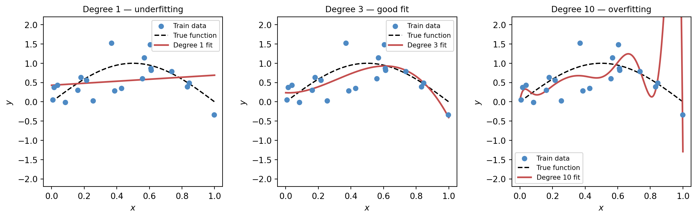
To make this concrete, consider fitting polynomial curves to noisy data from the function y = \sin(\pi x) + \varepsilon, where \varepsilon \sim \mathcal{N}(0, 0.3^2). With a degree-1 polynomial (a straight line), the model cannot follow the curve’s shape at all. It misses the genuine nonlinearity. With a degree-3 polynomial, the curve bends in the right directions and recovers the main signal. With a degree-10 polynomial, the model has enough freedom to pass through or near every training point — but between those points it oscillates wildly. On new data drawn from the same distribution, the degree-10 model performs far worse than the degree-3 model, even though it fits the training set better.

The language can sound informal, but the underlying issue is exact: how much of the variation in the data reflects durable signal, and how much is local noise?

Code

import numpy as np
import matplotlib.pyplot as plt

rng = np.random.default_rng(17)
n = 20
x_train = np.sort(rng.uniform(0, 1, n))
y_train = np.sin(np.pi * x_train) + rng.normal(0, 0.3, n)
x_true = np.linspace(0, 1, 300)
y_true = np.sin(np.pi * x_true)

degrees = [1, 3, 10]
titles = ['Degree 1 — underfitting', 'Degree 3 — good fit', 'Degree 10 — overfitting']

fig, axes = plt.subplots(1, 3, figsize=(12, 4))

for ax, deg, title in zip(axes, degrees, titles):
    coeffs = np.polyfit(x_train, y_train, deg)
    y_fit = np.polyval(coeffs, x_true)

    ax.scatter(x_train, y_train, color='#4e8ac4', zorder=4, s=30, label='Train data')
    ax.plot(x_true, y_true, 'k--', linewidth=1.5, label='True function')
    ax.plot(x_true, y_fit, color='#c44e4e', linewidth=2, label=f'Degree {deg} fit')
    ax.set_ylim(-2.2, 2.2)
    ax.set_xlabel('$x$')
    ax.set_ylabel('$y$')
    ax.set_title(title, fontsize=10)
    ax.legend(fontsize=8)

fig.tight_layout(pad=2.0)
plt.show()

Figure 5.1: Three polynomial fits to the same 20 noisy observations from y = \sin(\pi x) + \varepsilon. Degree 1 underfits (too rigid). Degree 3 fits well (right amount of flexibility). Degree 10 overfits (memorises noise).

5.7 Bias-variance tradeoff

The underfitting-overfitting tension has a precise mathematical form. For a given test point x_0, the expected squared prediction error decomposes as

\mathbb{E}\!\left[(y - \hat{f}(x_0))^2\right] = \underbrace{\bigl(\mathbb{E}[\hat{f}(x_0)] - f(x_0)\bigr)^2}_{\text{Bias}^2} + \underbrace{\mathrm{Var}\!\left[\hat{f}(x_0)\right]}_{\text{Variance}} + \underbrace{\sigma^2}_{\text{Irreducible}}.

Bias measures how far the average prediction of the model family is from the true value. A straight line fitted to sine data will always miss, no matter how much data we collect — that gap is systematic bias.

Variance measures how much the fitted model changes when the training set changes. A degree-10 polynomial fitted to 20 points is highly sensitive to which 20 points we happened to draw. Small changes in the sample produce wild swings in the fitted curve.

Irreducible error \sigma^2 is the noise in the data itself, independent of the model.

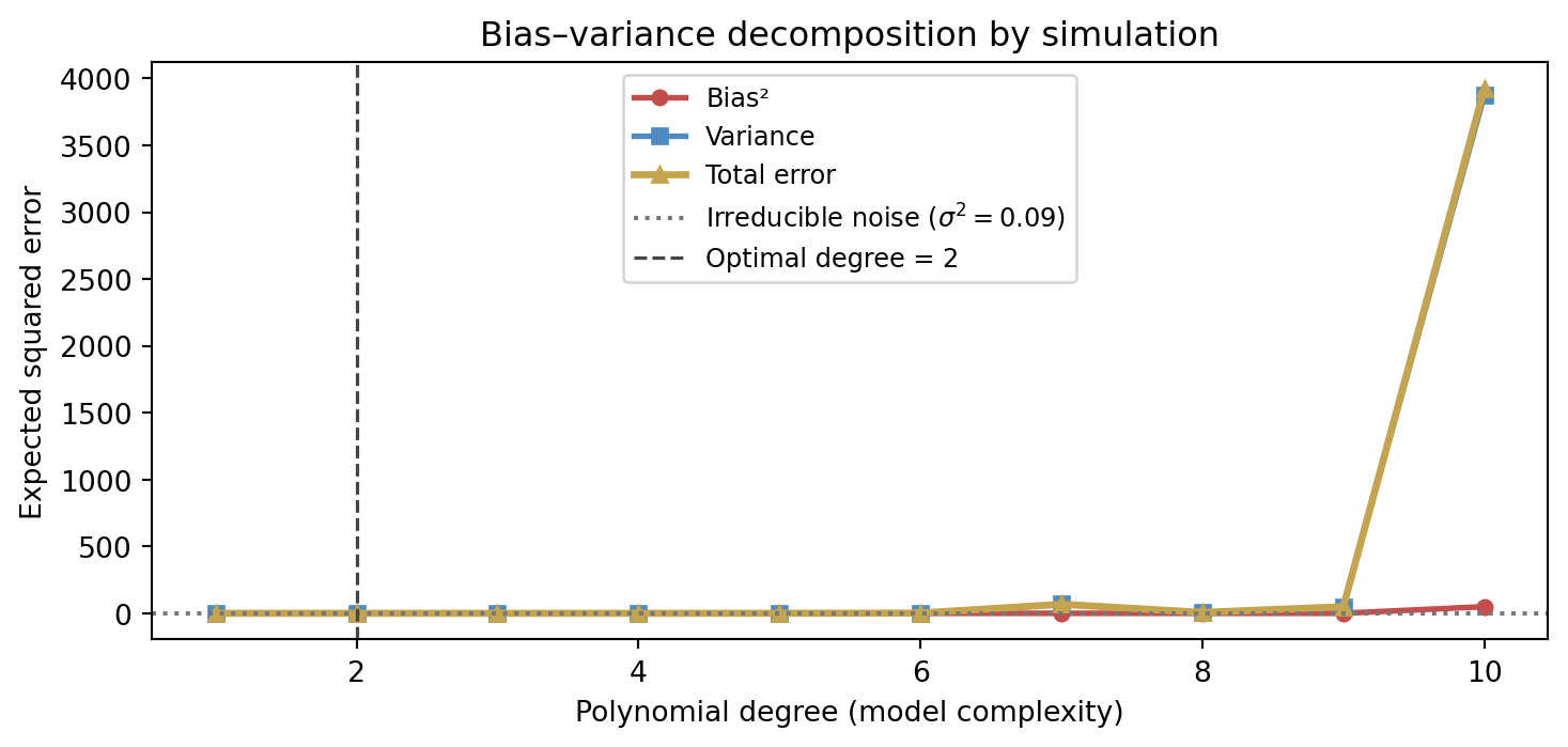
Simple models have high bias and low variance. Complex models have low bias and high variance. The optimal complexity minimises their sum (plus the fixed noise floor). This is not a metaphor — it can be computed by simulation.

The figure below estimates all three quantities by generating many training sets from the same process, fitting polynomials of each degree, and averaging. No external library is needed: the decomposition is computed directly from the simulation.

Code

import numpy as np
import matplotlib.pyplot as plt

rng = np.random.default_rng(99)

def true_f(x):
    return np.sin(np.pi * x)

sigma = 0.3
n_train = 20
n_sims = 200
x_test = np.linspace(0.05, 0.95, 50)
y_test_true = true_f(x_test)
degrees = np.arange(1, 11)

bias2_list = []
var_list = []

for deg in degrees:
    preds = np.zeros((n_sims, len(x_test)))
    for s in range(n_sims):
        x_tr = np.sort(rng.uniform(0, 1, n_train))
        y_tr = true_f(x_tr) + rng.normal(0, sigma, n_train)
        coeffs = np.polyfit(x_tr, y_tr, deg)
        preds[s] = np.polyval(coeffs, x_test)
    mean_pred = preds.mean(axis=0)
    bias2 = np.mean((mean_pred - y_test_true) ** 2)
    variance = np.mean(preds.var(axis=0))
    bias2_list.append(bias2)
    var_list.append(variance)

bias2_arr = np.array(bias2_list)
var_arr = np.array(var_list)
total = bias2_arr + var_arr + sigma ** 2

opt_deg = degrees[np.argmin(total)]

fig, ax = plt.subplots(figsize=(8, 4))
ax.plot(degrees, bias2_arr, color='#c44e4e', linewidth=2, marker='o', markersize=5,
        label='Bias²')
ax.plot(degrees, var_arr, color='#4e8ac4', linewidth=2, marker='s', markersize=5,
        label='Variance')
ax.plot(degrees, total, color='#c5a44e', linewidth=2.5, marker='^', markersize=5,
        label='Total error')
ax.axhline(sigma ** 2, color='#777', linestyle=':', linewidth=1.5,
           label=f'Irreducible noise ($\\sigma^2={sigma**2:.2f}$)')
ax.axvline(opt_deg, color='#444', linestyle='--', linewidth=1.2,
           label=f'Optimal degree = {opt_deg}')
ax.set_xlabel('Polynomial degree (model complexity)')
ax.set_ylabel('Expected squared error')
ax.set_title('Bias–variance decomposition by simulation')
ax.legend(fontsize=9)

fig.tight_layout(pad=2.0)
plt.show()

Figure 5.2: Bias–variance decomposition estimated by simulation across polynomial degrees 1–10. The optimal degree minimises total expected error. Irreducible noise sets the floor.

5.8 Regularisation as disciplined simplification

One of the healthiest ideas in statistical learning is regularisation.

Instead of asking the model only to fit the data well, we also ask it to remain simple in a chosen sense. The simplicity might mean smaller coefficients, fewer effective degrees of freedom, smoother functions, or less extreme decision boundaries.

That is not a cosmetic preference. It is a mathematical way of expressing the belief that wild explanations of limited data should be treated with suspicion.

Ridge regression adds a penalty on the squared magnitude of the coefficients. For a linear model with parameters \beta, the penalised objective is

J(\beta) = \|y - X\beta\|^2 + \lambda \|\beta\|^2,

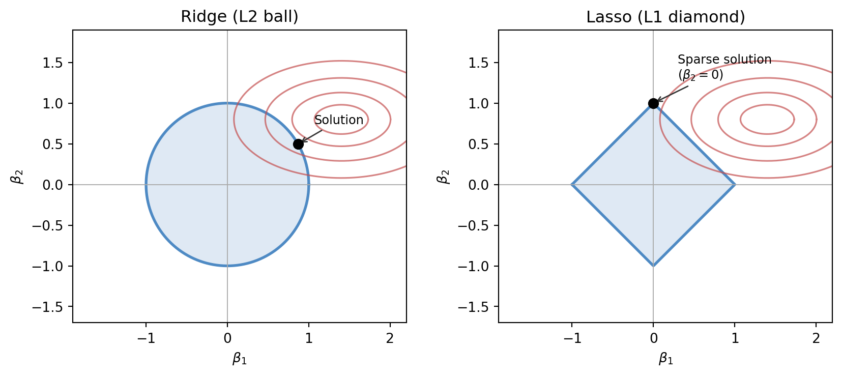
where \lambda \geq 0 controls the strength of the penalty. This has a closed form: the ridge estimator is \hat{\beta} = (X^\top X + \lambda I)^{-1} X^\top y. As \lambda increases, the coefficients shrink toward zero but none are exactly zeroed. The constraint set in coefficient space is a sphere (L2 ball).

Lasso regression replaces the squared-norm penalty with an absolute-value penalty:

J(\beta) = \|y - X\beta\|^2 + \lambda \|\beta\|_1.

The constraint set is now a diamond (L1 ball). The geometry of the diamond has corners on the coordinate axes. When loss contours meet the constraint set at a corner, the solution has an exact zero coefficient. This is why lasso produces sparse solutions — it effectively selects features — while ridge does not.

The figure below shows this geometry. On the left, an L2 ball and elliptical loss contours; the optimum lies on the smooth surface of the ball, not at a special point. On the right, an L1 diamond; the elliptical contours are more likely to contact the diamond at a corner, where one coefficient is exactly zero.

Code

import numpy as np
import matplotlib.pyplot as plt

fig, axes = plt.subplots(1, 2, figsize=(9, 4))

theta = np.linspace(0, 2 * np.pi, 300)

for ax, title, shape in zip(axes, ['Ridge (L2 ball)', 'Lasso (L1 diamond)'],
                             ['circle', 'diamond']):
    if shape == 'circle':
        bx = np.cos(theta)
        by = np.sin(theta)
    else:
        t = np.linspace(-1, 1, 300)
        bx = np.concatenate([t, t[::-1]])
        by = np.concatenate([1 - np.abs(t), -(1 - np.abs(t))])

    ax.fill(bx, by, alpha=0.18, color='#4e8ac4')
    ax.plot(bx, by, color='#4e8ac4', linewidth=2)

    cx, cy = 1.4, 0.8
    for level in [0.6, 1.1, 1.7, 2.4]:
        ell_x = cx + level * np.cos(theta) * 0.55
        ell_y = cy + level * np.sin(theta) * 0.30
        ax.plot(ell_x, ell_y, color='#c44e4e', linewidth=1.2, alpha=0.7)

    if shape == 'circle':
        ang = np.arctan2(cy - 0, cx - 0)
        px = np.cos(ang)
        py = np.sin(ang)
        ax.plot(px, py, 'ko', markersize=7, zorder=5)
        ax.annotate('Solution', (px, py), xytext=(px + 0.2, py + 0.25),
                    fontsize=9, arrowprops=dict(arrowstyle='->', color='#333'))
    else:
        ax.plot(0, 1, 'ko', markersize=7, zorder=5)
        ax.annotate('Sparse solution\n($\\beta_2 = 0$)', (0, 1),
                    xytext=(0.3, 1.3), fontsize=9,
                    arrowprops=dict(arrowstyle='->', color='#333'))

    ax.axhline(0, color='#aaa', linewidth=0.7)
    ax.axvline(0, color='#aaa', linewidth=0.7)
    ax.set_xlim(-1.9, 2.2)
    ax.set_ylim(-1.7, 1.9)
    ax.set_xlabel('$\\beta_1$')
    ax.set_ylabel('$\\beta_2$')
    ax.set_title(title)
    ax.set_aspect('equal')

fig.tight_layout(pad=2.0)
plt.show()

Figure 5.3: Regularisation geometry. Left: ridge (L2) — smooth ball, solution at a generic point on the boundary. Right: lasso (L1) — diamond, solution at a corner, forcing one coefficient to zero.

Later chapters will show regularisation appearing in many forms — weight decay in neural networks, early stopping, dropout — but its spirit is already visible here: fitting is never the whole story.

5.9 A modelling lens for the rest of the book

Statistical learning sits in the middle of the book because it teaches a habit that the later AI chapters depend on. We learn to ask:

what is the prediction task?
what kind of uncertainty is present?
what structure is signal and what structure is noise?
what constraints keep the model honest enough to generalise?

These questions will return in optimisation, representation learning, probabilistic modelling, and neural networks.

5.10 Optional viewpoints

quality control
sports or environmental forecasting
baseline predictive systems in operations

What to try

Adjust POLY_DEGREE from 1 to 12 to see how training and validation error diverge as complexity grows. Change LAMBDA (the regularisation strength) to see how penalising large coefficients can recover better validation performance at high degree.

import numpy as np
import matplotlib
matplotlib.use('Agg')
import matplotlib.pyplot as plt
import io, base64

# --- Try changing these parameters ---
POLY_DEGREE = 5
LAMBDA = 0.01

rng = np.random.default_rng(42)
n_total = 60
x_all = np.sort(rng.uniform(0, 1, n_total))
y_all = np.sin(np.pi * x_all) + rng.normal(0, 0.3, n_total)

n_train = 40
x_tr, y_tr = x_all[:n_train], y_all[:n_train]
x_val, y_val = x_all[n_train:], y_all[n_train:]

def vander(x, deg):
    return np.column_stack([x ** d for d in range(deg + 1)])

V_tr = vander(x_tr, POLY_DEGREE)
V_val = vander(x_val, POLY_DEGREE)

reg_matrix = LAMBDA * np.eye(POLY_DEGREE + 1)
reg_matrix[0, 0] = 0
beta = np.linalg.solve(V_tr.T @ V_tr + reg_matrix, V_tr.T @ y_tr)

train_mse = np.mean((y_tr - V_tr @ beta) ** 2)
val_mse = np.mean((y_val - V_val @ beta) ** 2)

x_plot = np.linspace(0, 1, 300)
V_plot = vander(x_plot, POLY_DEGREE)
y_plot = V_plot @ beta

train_errs = []
val_errs = []
degrees = np.arange(1, 13)
for deg in degrees:
    Vtr = vander(x_tr, deg)
    Vvl = vander(x_val, deg)
    reg = LAMBDA * np.eye(deg + 1)
    reg[0, 0] = 0
    b = np.linalg.solve(Vtr.T @ Vtr + reg, Vtr.T @ y_tr)
    train_errs.append(np.mean((y_tr - Vtr @ b) ** 2))
    val_errs.append(np.mean((y_val - Vvl @ b) ** 2))

fig, axes = plt.subplots(1, 2, figsize=(9, 4))

ax = axes[0]
ax.scatter(x_tr, y_tr, color='#4e8ac4', s=25, alpha=0.8, label='Train')
ax.scatter(x_val, y_val, color='#c5a44e', s=25, alpha=0.8, label='Validation')
ax.plot(x_plot, np.sin(np.pi * x_plot), 'k--', linewidth=1.5, label='True')
ax.plot(x_plot, y_plot, color='#c44e4e', linewidth=2,
        label=f'Degree {POLY_DEGREE} fit')
ax.set_xlabel('$x$')
ax.set_ylabel('$y$')
ax.set_title(f'Fit  |  Train MSE={train_mse:.3f}  Val MSE={val_mse:.3f}')
ax.legend(fontsize=8)

ax2 = axes[1]
ax2.plot(degrees, train_errs, color='#4e8ac4', linewidth=2, marker='o',
         markersize=5, label='Train MSE')
ax2.plot(degrees, val_errs, color='#c44e4e', linewidth=2, marker='s',
         markersize=5, label='Validation MSE')
ax2.axvline(POLY_DEGREE, color='#c5a44e', linestyle='--', linewidth=1.5,
            label=f'Current degree={POLY_DEGREE}')
ax2.set_xlabel('Polynomial degree')
ax2.set_ylabel('MSE')
ax2.set_title(f'Error curves  ($\\lambda={LAMBDA}$)')
ax2.legend(fontsize=8)

fig.tight_layout(pad=2.0)

buf = io.BytesIO()
fig.savefig(buf, format='png', dpi=96, bbox_inches='tight')
buf.seek(0)
img_b64 = base64.b64encode(buf.read()).decode()
print(f'<img src="data:image/png;base64,{img_b64}" style="max-width:100%">')

5.11 Exercises

MSE decomposition. Show analytically that \mathbb{E}[(y - \hat{y})^2] = \text{Bias}^2 + \text{Variance} + \sigma^2 by expanding y = f(x) + \varepsilon and \hat{y} = \hat{f}(x), where \varepsilon has mean zero and variance \sigma^2 and is independent of \hat{f}.
Polynomial degree selection. For a synthetic dataset of your choice drawn from a nonlinear function with noise, split the data 70/30 and compute validation MSE for polynomial degrees 1 through 8. Plot the curve and identify the degree that minimises validation error. How does this degree change if you double the noise level?
Ridge estimator. Starting from the penalised objective J(\beta) = \|y - X\beta\|^2 + \lambda\|\beta\|^2, differentiate with respect to \beta, set to zero, and derive the ridge estimator \hat{\beta} = (X^\top X + \lambda I)^{-1} X^\top y. Show that when \lambda > 0 the matrix X^\top X + \lambda I is always invertible, and explain why this makes ridge more numerically stable than ordinary least squares when features are nearly collinear.
Regularisation path. Describe what happens to the ridge coefficients as \lambda \to 0 and as \lambda \to \infty. Then answer the same question for lasso. In the lasso case, which coefficients reach zero first as \lambda increases, and what does this tell us about feature selection?